Enriching Offline Reinforcement Learning Algorithms in ReinforcementLearning.jl

This is the phase 2 technical report of the summer OSPP project Enriching Offline Reinforcement Learning Algorithms in ReinforcementLearning.jl. The report is split into the following parts: Project Information and Completed Work.

Table of content

Technical Report

Technical Report

This technical report is the second phase technical report of Project "Enriching Offline Reinforcement Learning Algorithms in ReinforcementLearning.jl" in OSPP. It includes two components: project information and completed work.

Project Information

Project name: Enriching Offline Reinforcement Learning Algorithms in ReinforcementLearning.jl
Scheme Description: Recent advances in offline reinforcement learning make it possible to turn reinforcement learning into a data-driven discipline, such that many effective methods from the supervised learning field could be applied. Until now, the only offline method provided in ReinforcementLearning.jl is Behavior Cloning (BC). We'd like to have more algorithms added like Batch Constrain deep Q-Learning (BCQ), Conservative Q-Learning (CQL). It is expected to implement at least three to four modern offline RL algorithms.
Time planning: the following is a relatively simple time table.

Date	Work
Prior - June 30	Preliminary research, including algorithm papers, ReinforcementLearning.jl library code, etc.
The first phase
July1 - July15	Design and build the framework of offline RL.
July16 - July31	Implement and experiment offline DQN and offline SAC as benchmark.
August1 - August15	Write build-in documentation and technical report. Implement and experiment CRR.
The second phase
August16 - August31	Implement and experiment PLAS.
September1 - September15	Research, implement and experiment new SOTA offline RL algorithms.
September16 - September30	Write build-in documentation and technical report. Buffer for unexpected delay.
After project	Carry on fixing issues and maintaining implemented algorithms.

Completed Work

It summarizes all the results of the second phase.

Offline RL algorithms

In the second phase, we finished the offline RL algorithms: BCQ, Discrete-BCQ, BEAR(UWAC), FisherBRC. CRR and PLAS are detailed in the report of the first phase. Except for algorithms in discrete action space (such as Discrete-BCQ, Discrete-CRR), all algorithms can run on CPU and GPU, because CartesianIndex is not supported in GPU.

BCQ

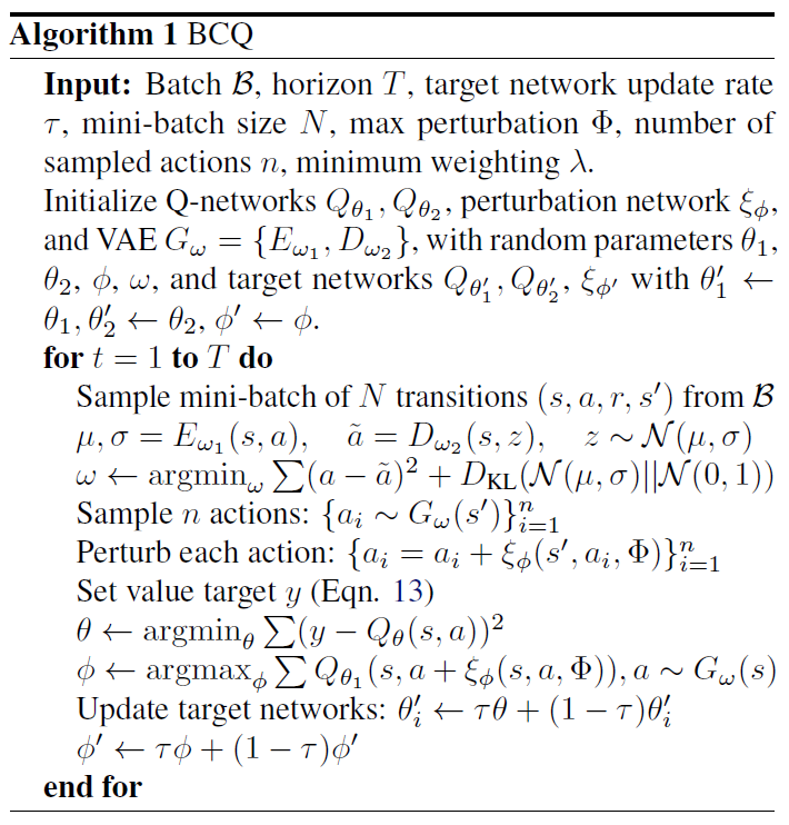
Batch-Constrained deep Q-Learning (BCQ) uses distribution matching to constrain policy. The pseudocode of BCQ:

BCQ needs to train a VAE to sample actions based on the next state. We train VAE for a period of time, and then train VAE and BCQ learner simultaneously to ensure the quality of the generated actions. When sampling actions, we randomly samples hidden states instead of generating hidden states in PLAS. Therefore, we re-implement decode function in VAE:

function decode(rng::AbstractRNG, model::VAE, state, z=nothing; is_normalize::Bool=true)
    if z === nothing
        # In BCQ case. In PLAS case if z !== nothing.
        z = clamp.(randn(rng, Float32, (model.latent_dims, size(state)[2:end]...)), -0.5f0, 0.5f0)
        z = send_to_device(device(model), z)
    end
    a = model.decoder(vcat(state, z))
    if is_normalize
        a = tanh.(a)
    end
    return a
end

And it needs a perturbation network:

Base.@kwdef struct PerturbationNetwork{N}
    base::N
    ϕ::Float32 = 0.05f0
end

Perturbation network is used to increase the robustness of the action:

function (model::PerturbationNetwork)(state, action)
    x = model.base(vcat(state, action))
    x = model.ϕ * tanh.(x)
    clamp.(x + action, -1.0f0, 1.0f0)
end

Please refer to this link for specific code (link). The brief function parameters are as follows:

mutable struct BCQLearner{BA1, BA2, BC1, BC2, V} <: AbstractLearner
    ### Omit other parameters
    policy::BA1
    target_policy::BA2
    qnetwork1::BC1
    qnetwork2::BC2
    target_qnetwork1::BC1
    target_qnetwork2::BC2
    vae::V
    p::Int
    start_step::Int
end

In BCQ, we use PerturbationNetwork: $\pi(s,a)\rightarrow a$ to model policy and use $Q(s,a)$ to model Q-network.

p is a hyper-parameter used for repeating states to obtain better Q estimation. For example, BCQ repeats states and obtains the actions and Q-values. Then it chooses an action with the highest Q-value.

function (l::BCQLearner)(env)
    s = send_to_device(device(l.policy), state(env))
    s = Flux.unsqueeze(s, ndims(s) + 1)
    s = repeat(s, outer=(1, 1, l.p))
    action = l.policy(s, decode(l.vae.model, s))
    q_value = l.qnetwork1(vcat(s, action))
    idx = argmax(q_value)
    action[idx]
end

start_step represents the steps to train VAE alone.

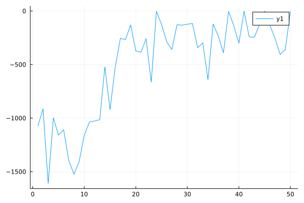
Performance curve of BCQ algorithm in Pendulum (start_step=1000):

Discrete BCQ

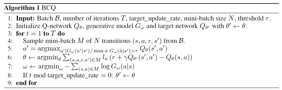
Discrete BCQ is a simple offline RL algorithm in discrete action space. Its pseudocode is as follow:

The core of Discrete BCQ is calculating a mask of actions. We calculate the probability of actions in a given state and divide it by the maximum probability value. Then, we compare this value with the threshold. If this value is less than the threshold, the corresponding action will not be selected.

prob = softmax(learner.approximator.actor(s), dims=1)
mask = Float32.((prob ./ maximum(prob, dims=1)) .> learner.threshold)
new_q = q .* mask .+ (1.0f0 .- mask) .* -1f8

Please refer to this link for specific code (link). The brief function parameters are as follows:

mutable struct BCQDLearner{Aq, At} <: AbstractLearner
    ### Omit other parameters
    approximator::Aq
    target_approximator::At
    θ::Float32
    threshold::Float32
end

In Discrete BCQ, we use the Actor-Critic structure. The Critic is modeled as $Q(s,\cdot)$ , and the Actor is modeled as $L(s,\cdot)$ (likelihood of the state).

θ is the regularization coefficient. When calculating the loss in Discrete BCQ, it uses the likelihood of the state to regularize:

logit = AC.actor(s)
actor_loss + critic_loss + θ * mean(logit .^ 2)

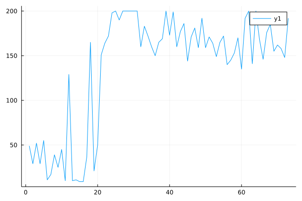
Performance curve of Discrete BCQ algorithm in CartPole:

BEAR & UWAC

Bootstrapping error accumulation reduction (BEAR) is a policy-constraint method, which uses support constrain instead of distribution matching in BCQ. Its pseudocode is as follow:

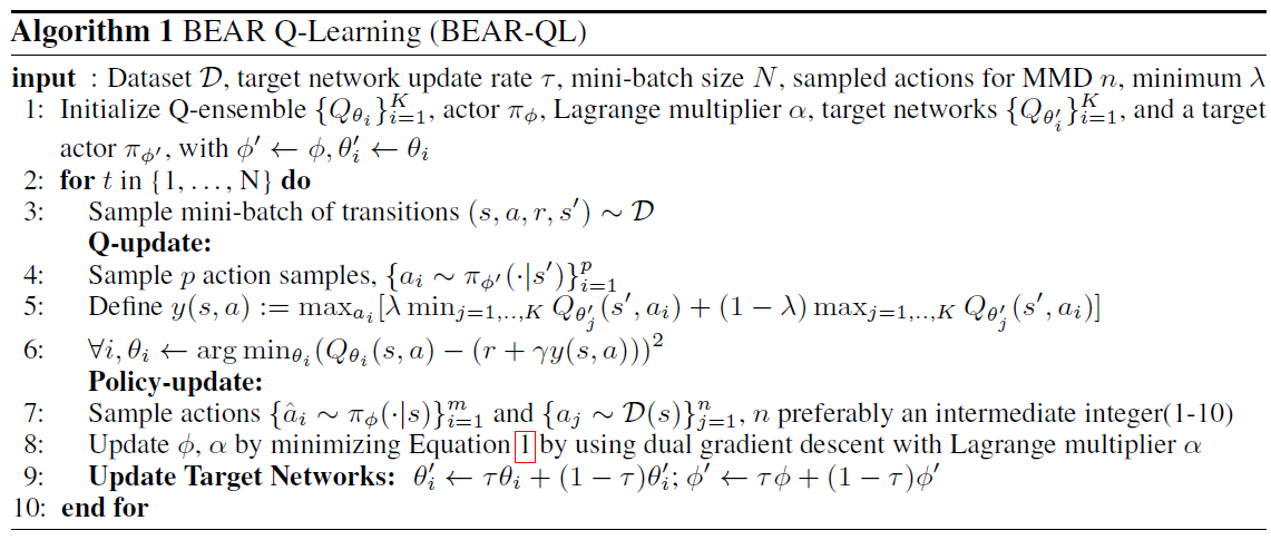
The equation 1:

\pi_\phi := \max_{\pi \in \triangle_{|S|}}\mathbb{E}_{s\in \mathcal{D}}\mathbb{E}_{a\sim\pi(\cdot|s)}\big[\min_{j=1,\cdots,K}\hat{Q}_j(s,a)\big] \\ s.t. \mathbb{E}_{s\in\mathcal{D}}[{\rm MMD}(\mathcal{D}(s),\pi(\cdot|s))]\leq \varepsilon

The Actor update is the main improvement part of BEAR. We need to train a VAE to simulate sampling action from the dataset. The training of the VAE and the learner are synchronized. Then we sample action by the Actor and calculate maximum mean discrepancy (MMD) loss:

function maximum_mean_discrepancy_loss(raw_sample_action, raw_actor_action, type::Symbol, mmd_σ::Float32=10.0f0)
    A, B, N = size(raw_sample_action)
    diff_xx = reshape(raw_sample_action, A, B, N, 1) .- reshape(raw_sample_action, A, B, 1, N)
    diff_xy = reshape(raw_sample_action, A, B, N, 1) .- reshape(raw_actor_action, A, B, 1, N)
    diff_yy = reshape(raw_actor_action, A, B, N, 1) .- reshape(raw_actor_action, A, B, 1, N)
    diff_xx = calculate_sample_distance(diff_xx, type, mmd_σ)
    diff_xy = calculate_sample_distance(diff_xy, type, mmd_σ)
    diff_yy = calculate_sample_distance(diff_yy, type, mmd_σ)
    mmd_loss = sqrt.(diff_xx .+ diff_yy .- 2.0f0 .* diff_xy .+ 1.0f-6)
end

The loss of actor is:

J=-Q_{\hat{\theta}}(s,a) + \alpha \times {\rm MMD}(\mathcal{D}(s),\pi(\cdot|s))

Besides, lagrangian multiplier $\alpha$ needs to be updated synchronously:

J=-Q_{\hat{\theta}}(s,a) + \alpha \times ({\rm MMD}(\mathcal{D}(s),\pi(\cdot|s))-\varepsilon)

Please refer to this link for specific code (link). The brief function parameters are as follows:

mutable struct BEARLearner{BA1, BA2, BC1, BC2, V, L} <: AbstractLearner
    ### Omit other parameters
    policy::BA1
    target_policy::BA2
    qnetwork1::BC1
    qnetwork2::BC2
    target_qnetwork1::BC1
    target_qnetwork2::BC2
    vae::V
    log_α::L
    ε::Float32
    p::Int
    max_log_α::Float32
    min_log_α::Float32
    sample_num::Int
    kernel_type::Symbol
    mmd_σ::Float32
end

In BEAR, we use $Q(s, a)$ to model the Q-network and use a gaussian network to model the policy. log_α is a Lagrange multiplier implemented by a NeuralNetworkApproximator.

ε is used to update the Lagrangian multiplier. p is a hyper-parameter like BCQ. max_log_α and min_log_α are used to clamp the log_α. sample_num represents how many samples we sample to calculate MMD loss. mmd_σ is used to adjust the size of MMD loss. kernel_type=:laplacian/:gaussian represents what method we use to calculate MMD loss:

function calculate_sample_distance(diff, type::Symbol, mmd_σ::Float32)
    if type == :gaussian
        diff = diff .^ 2
    elseif type == :laplacian
        diff = abs.(diff)
    else
        error("Wrong parameter.")
    end
    return vec(mean(exp.(-sum(diff, dims=1) ./ (2.0f0 * mmd_σ)), dims=(3, 4)))
end

Performance curve of BEAR algorithm in Pendulum:

Uncertainty Weighted Actor-Critic (UWAC) is an improvement of BEAR. It can be implemented by adding Dropout in BEAR's Q network.

FisherBRC

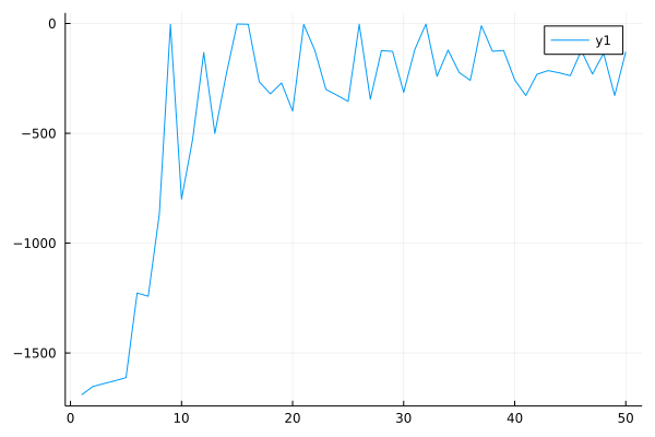
FisherBRC is a policy-constraint offline RL algorithm, which uses Fisher distance to constrain policy. The pseudocode of FisherBRC:

Firstly, it needs to pre-train a behavior policy $\mu$ using Behavior Cloning. In official python implementation, it adds an entropy term in the negative log-likelihood of actions in a given state. Mathematical formulation:

\mathcal{L}(\mu) = \mathbb{E}[-\log \mu(s|a) + \alpha \mathcal{H}(\mu)]

Besides, it automatically adjusts entropy term like SAC:

J(\alpha) = -\alpha \mathbb{E}_{a_t\sim \mu_t}[\log\mu(a_t|s_t) + \bar{\mathcal{H}}]

Where $\bar{\mathcal{H}}$ is target entropy. But in ReinforcementLearningZoo.jl, BehaviorCloningPolicy does not contain the entropy term and does not support continuous action space. So, we define EntropyBC:

mutable struct EntropyBC{A<:NeuralNetworkApproximator}
    policy::A
    α::Float32
    lr_alpha::Float32
    target_entropy::Float32
    # Logging
    policy_loss::Float32
end

Users only need to set parameter policy and lr_alpha. policy usually uses a GaussianNetwork. lr_alpha is the learning rate of α, which is an entropy term. target_entropy is set to $-\dim(\mathcal{A})$ , and $\mathcal{A}$ is action space.

Afterward, the FisherBRC learner is updated. When updating Actor, it adds an entropy term in Q-value loss and automatically adjusts entropy. It updates Critic by this equation:

\min_\theta J(O_\theta + \log\mu(a|s)) + \lambda \mathbb{E}_{s\sim D, a\sim \pi_\phi(\cdot|s)}[\|\nabla_a O_\theta(s,a)\|^2]

There are a few key concepts that need to be introduced. $J$ is the standard Q-value loss function. $O_\theta(s,a)$ is offset network:

Q_\theta(s,a) = O_\theta(s,a) + \log\mu(a|s)

Instead of $Q_\theta(s,a)$ , $O_\theta(s,a)$ will provide a richer representation of Q-values. However, this parameterization can potentially put us back in the fully-parameterized $Q_\theta$ regime of vanilla actor critic. So it uses a gradient penalty regularizer of the form $\|\nabla_a O_\theta(s,a)\|$ . The implementation is as follows:

a_policy = l.policy(l.rng, s; is_sampling=true)
q_grad_1 = gradient(Flux.params(l.qnetwork1)) do
    q1 = l.qnetwork1(q_input) |> vec
    q1_grad_norm = gradient(Flux.params([a_policy])) do 
        q1_reg = mean(l.qnetwork1(vcat(s, a_policy)))
    end
    reg = mean(q1_grad_norm[a_policy] .^ 2)
    loss = mse(q1 .+ log_μ, y) + l.f_reg * reg  # y is target value
end

Please refer to this link for specific code (link). The brief function parameters are as follows:

mutable struct FisherBRCLearner{BA1, BC1, BC2} <: AbstractLearner
    ### Omit other parameters
    policy::BA1
    behavior_policy::EntropyBC
    qnetwork1::BC1
    qnetwork2::BC2
    target_qnetwork1::BC1
    target_qnetwork2::BC2
    α::Float32
    f_reg::Float32
    reward_bonus::Float32
    pretrain_step::Int
    lr_alpha::Float32
    target_entropy::Float32
end

In FisherBRC, policy is modeled as gaussian network and Q-network is modeled as $O(s,a)$ .

f_reg is the regularization parameter of $\|\nabla_a O_\theta(s,a)\|$ . reward_bonus is generally set to 5, which is added in the reward to improve performance. pretrain_step is used for pre-training behavior_policy. α, lr_alpha and target_entropy are parameters used to add an entropy term and automatically adjust the entropy.

Performance curve of FisherBRC algorithm in Pendulum (pertrain_step=100):

Offline RL experiments

To show performance of the above algorithms, we add some built-in experiments in ReinforcementLearningExperiments.jl.

If it is an algorithm on the continuous action space, we test it in Pendulum, otherwise we test it on CartPole.

We collect the dataset by gen_JuliaRL_dataset function (source):

struct JuliaRLTransition
    state
    action
    reward
    terminal
    next_state
end

function gen_JuliaRL_dataset(alg::Symbol, env::Symbol, type::AbstractString; dataset_size::Int)
    dataset_ex = Experiment(
            Val(:GenDataset),
            Val(alg),
            Val(env),
            type;
            dataset_size = dataset_size)
    
    run(dataset_ex)

    dataset = []
    s, a, r, t = dataset_ex.policy.trajectory.traces
    for i in 1:dataset_size
        push!(dataset, JuliaRLTransition(s[:, i], a[i], r[i], t[i], s[:, i+1]))
    end
    dataset
end

Specifically, we first run the built-in data collection experiment. For CartPole environment, we use BasicDQN to collect the dataset. For Pendulum, SAC is used. Then we turn the trajectory into a vector of JuliaRLTranstion.

We can run the offline RL experiments with the following commands (list all supported commands):

run(E`JuliaRL_BCQ_Pendulum(type)`)
run(E`JuliaRL_BCQD_CartPole(type)`)
run(E`JuliaRL_BEAR_Pendulum(type)`)
run(E`JuliaRL_CRR_Pendulum(type)`)
run(E`JuliaRL_CRR_CartPole(type)`)
run(E`JuliaRL_FisherBRC_Pendulum(type)`)
run(E`JuliaRL_PLAS_Pendulum(type)`)

type represents the method of collecting dataset, which can be random, medium or expert. random means dataset generated by the random agent, and medium uses an agent trained from scratch to convergence, and expert uses an agent that has converged. For example:

run(E`JuliaRL_BCQ_Pendulum(medium)`)

Conclusion

The implemented algorithms in this project contain most of the policy constraint methods in offline reinforcement learning (including distribution matching, support constrain, implicit constraint, behavior cloning). And these algorithms cover both discrete and continuous action spaces. Besides, we have them tested with various datasets, including random, medium, and expert.

Corrections

If you see mistakes or want to suggest changes, please create an issue in the source repository.