Enriching Offline Reinforcement Learning Algorithms in ReinforcementLearning.jl

This is the phase 1 technical report of the summer OSPP project Enriching Offline Reinforcement Learning Algorithms in ReinforcementLearning.jl used for mid-term evaluation. The report is split into the following parts: Project Information, Project Schedule and Future Plan.

Table of content

Technical Report

Technical Report

This technical report is the first evaluation report of Project "Enriching Offline Reinforcement Learning Algorithms in ReinforcementLearning.jl" in OSPP. It includes three components: project information, project schedule, future plan.

Project Information

Project name: Enriching Offline Reinforcement Learning Algorithms in ReinforcementLearning.jl
Scheme Description: Recent advances in offline reinforcement learning make it possible to turn reinforcement learning into a data-driven discipline, such that many effective methods from the supervised learning field could be applied. Until now, the only offline method provided in ReinforcementLearning.jl is Behavior Cloning (BC). We'd like to have more algorithms added like Batch Constrain Q-Learning (BCQ), Conservative Q-Learning (CQL). It is expected to implement at least three to four modern offline RL algorithms.
Time planning: the following is a relatively simple time table.

Date	Work
Prior - June 30	Preliminary research, including algorithm papers, ReinforcementLearning.jl library code, etc.
The first phase
July1 - July15	Design and build the framework of offline RL.
July16 - July31	Implement and experiment offline DQN and offline SAC as benchmark.
August1 - August15	Write build-in documentation and technical report. Implement and experiment CRR.
The second phase
August16 - August31	Implement and experiment PLAS.
September1 - September15	Research, implement and experiment new SOTA offline RL algorithms.
September16 - September30	Write build-in documentation and technical report. Buffer for unexpected delay.
After project	Carry on fixing issues and maintaining implemented algorithms.

Project Schedule

This part mainly introduces the results of the first phase.

Basic framework

To run and test the offline algorithm, we first implemented OfflinePolicy.

Base.@kwdef struct OfflinePolicy{L,T} <: AbstractPolicy
    learner::L
    dataset::T
    continuous::Bool
    batchsize::Int
end

This implementation of OfflinePolicy refers to QBasePolicy. It provides a parameter continuous to support different action space types, including continuous and discrete. learner is a specific algorithm for learning and providing policy. dataset and batchsize are used to sample data for learning.

Besides, we implement corresponding functions π, update! and sample. π is used to select the action, whose form is determined by the type of action space. update! can be used in two stages. In PreExperiment stage, we can call this function for pre-training algorithms with pretrain_step parameters. In PreAct stage, we call this function for training the learner. In function update!, we need to call function sample to sample a batch of data from the dataset. With the development of ReinforcementLearningDataset.jl, the sample function will be deprecated.

We can quickly call the offline version of the existing algorithms with almost no additional code with this framework. Therefore, the implementation and performance testing of offline DQN and offline SAC can be completed soon. For example:

offline_dqn_policy = OfflinePolicy(
    learner = DQNLearner(
        # Omit specific code
    ),
    dataset = dataset,
    continuous = false,
    batchsize = 64,
)

Therefore, we unify the parameter name in different algorithms so that different learners can be compatible with OfflinePolicy.

Useful Components

GaussianNetwork

GaussianNetwork models a Normal Distribution $\mathcal{N}(\mu,\sigma^2)$ , which is often used in tasks with continuous action space. It consists of three neural network chains:

Base.@kwdef struct GaussianNetwork{P,U,S}
    pre::P = identity
    μ::U
    logσ::S
    min_σ::Float32 = 0f0
    max_σ::Float32 = Inf32
end

We implement the evaluation function and inference function of GaussianNetwork. By evaluation function, given the state, then the mean and log-standard deviation are obtained. Furthermore, we can sample the action from distribution and get the probability of the action in a given state. When calling the inference function with parameter state and action, we get the likelihood of the action in a given state.

### Evaluation
function (model::GaussianNetwork)(state; is_sampling::Bool=false, is_return_log_prob::Bool=false)
    # Omit specific code
    if is_sampling
        if is_return_log_prob
            return tanh.(z), logp_π
        else
            return tanh.(z)
        end
    else
        return μ, logσ
    end
end
### Inference
function (model::GaussianNetwork)(state, action)
    # Omit specific code
    return logp_π
end

Variational Auto-Encoder (VAE)

In offline reinforcement learning tasks, VAE is often used to learn from datasets to approximate behavior policy.

The VAE we implemented contains two neural networks: encoder and decoder (link).

Base.@kwdef struct VAE{E, D}
    encoder::E
    decoder::D
end

In the encoding stage, it accepts input state and action and outputs the mean and standard deviation of the distribution. Afterward, the hidden action is obtained by sampling from the resulted distribution. In the decoding stage, state and hidden action are used as the input to reconstruct action.

During training, we call the vae_loss function to get the reconstruction loss and KL loss. The specific task determines the ratio of these two losses.

function vae_loss(model::VAE, state, action)
    # Omit specific code
    return recon_loss, kl_loss
end

In the specific algorithm, the functions that may need to be called are as follows:

### Encode + decode
function (model::VAE)(state, action)
    ### Omit specific code
    return a, μ, σ
end
### Decode
function decode(model::VAE, state, z)
    ### Omit specific code
    return a
end

Offline RL Algorithms

We used the existing algorithms and hooks to train the offline RL algorithm to create datasets in several environments (such as CartPole, Pendulum) for training. This work can guide the subsequent development of package ReinforcementLearningDataset.jl, for example:

gen_dataset("JuliaRL-CartPole-DQN", policy, env)

Benchmark

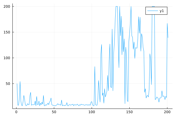
We implement and experiment with offline DQN (in discrete action space) and offline SAC (in continuous action space) as benchmarks. The performance of offline DQN in Cartpole environment:

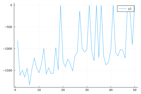
The performance of offline SAC in Pendulum environment:

Conservative Q-Learning (CQL)

CQL is an efficient and straightforward Q-value constraint method. Other offline RL algorithms can easily use this constraint to improve performance. Therefore, we implement CQL as a common component (link). For other algorithms, we only need to add CQL loss to their loss.

function calculate_CQL_loss(q_value, qa_value)
    cql_loss = mean(log.(sum(exp.(q_value), dims=1)) .- qa_value)
    return cql_loss
end
### DQN loss
gs = gradient(params(Q)) do
        q = Q(s)[a]
        loss = loss_func(G, q)
        ignore() do
            learner.loss = loss
        end
        loss + calculate_CQL_loss(Q(s), q)
    end

After adding CQL loss, the performance of offline DQN improve.

Currently, this function only supports discrete action space and CQL(H) method.

Critic Regularizer Regression (CRR)

CRR is a Behavior Cloning based method. To filter out bad actions and enables learning better policies from low-quality data, CRR utilizes the advantage function to regularize the learning objective of the actor. Pseudocode is as follows:

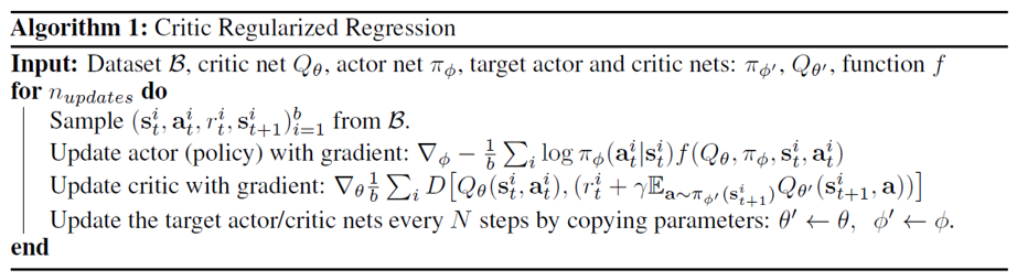
In different tasks, $f$ has different choices:

𝑓=\mathbb{I}[A_\theta(s,a)>0]\quad \mathnormal{or}\quad f=e^{A_\theta(s,a)/\beta}

We implemented discrete CRR and continuous CRR (link). The brief function parameters are as follows:

mutable struct CRRLearner{Aq, At, R} <: AbstractLearner
    ### Omit other parameters
    approximator::Aq # Actor-Critic
    target_approximator::At # Actor-Critic
    policy_improvement_mode::Symbol
    ratio_upper_bound::Float32
    beta::Float32
    advantage_estimator::Symbol
    m::Int
    continuous::Bool
end

In CRR, we use the Actor-Critic structure. In the case of discrete action space, the Critic is modeled as $Q(s,\cdot)$ , and the Actor is modeled as $L(s,\cdot)$ (likelihood of the state). In the case of continuous action space, we use $Q(s, a)$ to model the Critic, and use gaussian network to model the Actor.

Parameter continuous stands for the type of action space. policy_improvement_mode is the type of the weight function $f$ . If policy_improvement_mode=:binary, we use the first $f$ function. Otherwise, we use the second $f$ function, which needs parameter ratio_upper_bound (Upper bound of $f$ value) and beta. Besides, we provide two methods to estimate advantage function, specifing advantage_estimator=:mean/:max. In the discrete case, we can calculate $A(s,a)$ directly. In the continuous case, we need to sample m Q-values to calculate advantage function.

Different action spaces will also affect the implementation of the Actor-Critic. In the discrete case, the Actor outputs logits of all actions in a given state. Gaussian networks are used to model the Actor in the continuous case.

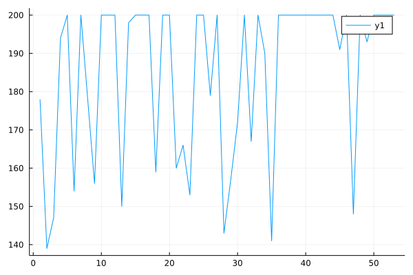
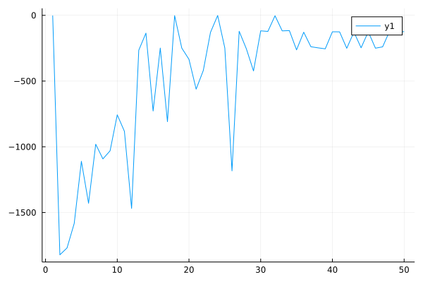
Performance curve of discrete CRR algorithm in CartPole:

Performance curve of continuous CRR algorithm in Pendulum:

Policy in the Latent Action Space (PLAS)

PLAS is a policy constrain method suitable for continuous control tasks. Unlike BCQ and BEAR, PLAS implicitly constrains the policy to output actions within the support of the behavior policy through the latent action space:

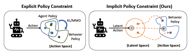
PLAS pre-trains a CVAE (Conditional Variational Auto-Encoder) to constrain policy. In the pre-training phase, PLAS samples state-action pairs to train CVAE. PLAS needs to learn a deterministic policy mapping state to latent action and then uses CVAE mapping latent action to action in the training phase. When PLAS mapping state or latent action, it needs to use tanh function to limit the output range.

The advantage of pre-training VAE is that it can accelerate the convergence, and it is easier to train when encountered with complex action spaces and import existing VAE models. Its pseudocode is as follows:

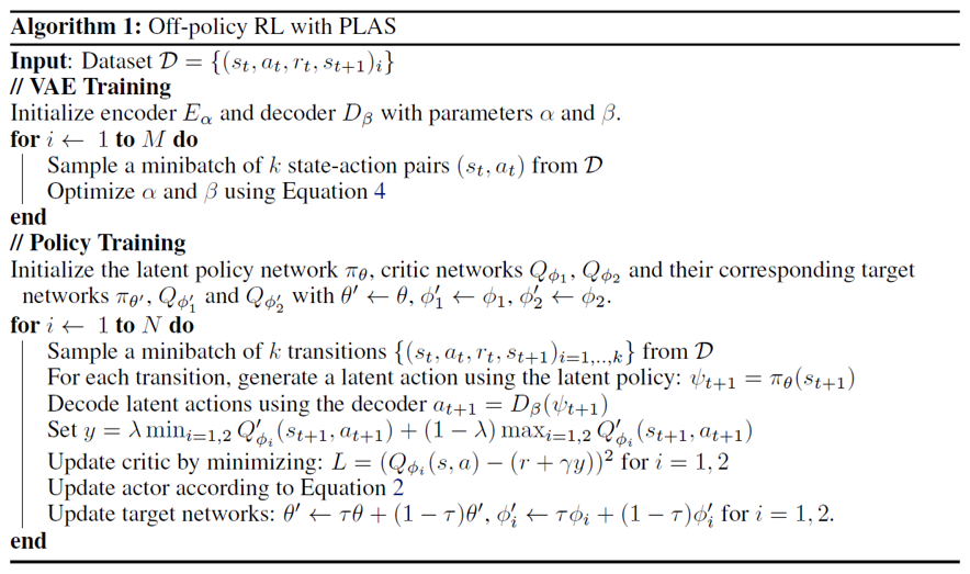
Please refer to this link for specific code (link). The brief function parameters are as follows:

mutable struct PLASLearner{BA1, BA2, BC1, BC2, V, R} <: AbstractLearner
    ### Omit other parameters
    policy::BA1
    target_policy::BA2
    qnetwork1::BC1
    qnetwork2::BC2
    target_qnetwork1::BC1
    target_qnetwork2::BC2
    vae::V
    λ::Float32
    pretrain_step::Int
end

In PLAS, Q-network is modeled as $Q(s, a)$ and policy is modeled as deterministic policy: $\pi(s)\rightarrow a_{latent}$ .

If the algorithm requires pre-training, please specify the parameter pretrain_step and function update!. We modified the run function and added an interface:

function (agent::Agent)(stage::PreExperimentStage, env::AbstractEnv)
    update!(agent.policy, agent.trajectory, env, stage)
end

function RLBase.update!(p::OfflinePolicy, traj::AbstractTrajectory, ::AbstractEnv, ::PreExperimentStage)
    l = p.learner
    if in(:pretrain_step, fieldnames(typeof(l)))
        println("Pretrain...")
        for _ in 1:l.pretrain_step
            inds, batch = sample(l.rng, p.dataset, p.batchsize)
            update!(l, batch)
        end
    end
end

In PLAS, we use conditional statements to select training components:

function RLBase.update!(l::PLASLearner, batch::NamedTuple{SARTS})
    if l.update_step == 0
        update_vae!(l, batch)
    else
        update_learner!(l, batch)
    end
end

λ is the parameter of clipped double Q-learning (used for Critic training), a small trick to reduce overestimation. Actor training uses the standard policy gradient method.

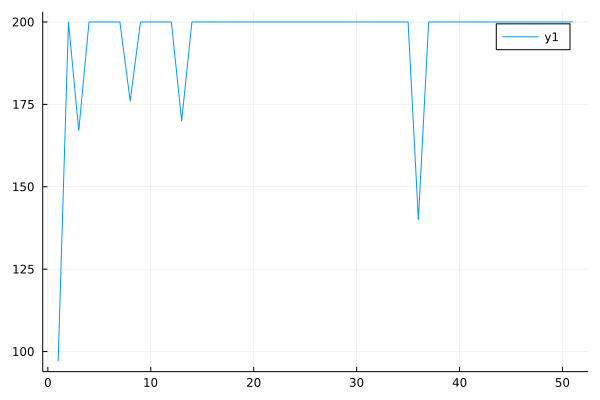
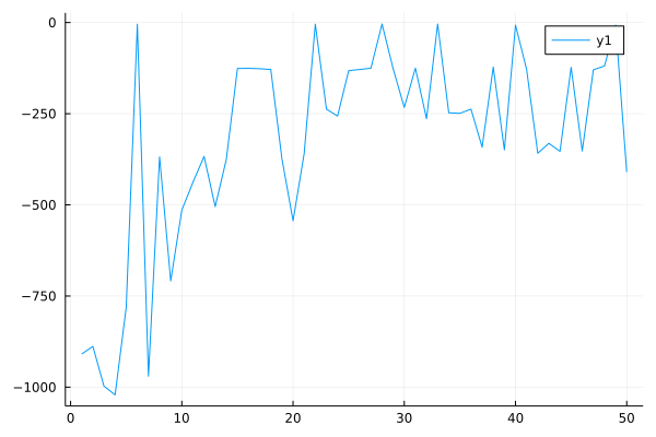
Performance curve of PLAS algorithm in Pendulum (pertrain_step=1000):

However, the action perturbation component in PLAS has not yet been completed and needs to be implemented in the second stage.

Other Work

In addition to the above work, we also did the following:

Add copyto function in ActorCritic. This function is needed to synchronize between target Actor-Critic and online Actor-Critic.
Add the tuning entropy component in SAC to improve performance.

Conclusion

During this process, we learn a lot:

Algorithm level. We researched more than a dozen top conference papers on offline reinforcement learning regions to implement more modern offline RL algorithms. Therefore, we understand the core problem of offline RL and how to solve the problem, as well as the shortcomings of the current method. This is of great benefit to our future research and work.
Code level. Implementing these algorithms allowed us to increase the code and debug capabilities in Julia programming. Besides, we learned a lot of knowledge about code specifications, version management, and git usage. These experiences can be of great help to future development.
Cooperation level. We must cooperate with everyone, including the mentor and other developers, to contribute to a public algorithm library. The ideas of the collaborators will give us a lot of inspiration.

Future Plan

The following is our future plan:

Date	Work
August16 - August23	Debug and finish CRR and PLAS.
August24 - August31	Read the paper and python code of UWAC.
September1 - September7	Implement and experiment UWAC.
September8 - September15	Read the paper and python code of FisherBRC.
September16 - September23	Implement and experiment FisherBRC.
September24 - September30	Write build-in documentation and technical report. Buffer for unexpected delay.
After project	Carry on fixing issues and maintain implemented algorithms.

Firstly, we need to fix bugs in continuous CRR and finish action perturbation component in PLAS. The current progress is slightly faster than the originally set progress, so we can implement more of the modern offline RL algorithms. The current plan includes UWAC and FisherBRC published on ICML'21. Here we briefly introduce these two algorithms:

Uncertainty Weighted Actor-Critic (UWAC). The algorithm is based on the improvement of BEAR. The authors adopt a practical and effective dropout-based uncertainty estimation method, Monte Carlo (MC) dropout, to identify and ignore OOD training samples, to introduce very little overhead over existing RL algorithms.
Fisher Behavior Regularized Critic (Fisher-BRC). The algorithm is based on the improvement of BRAC. The authors propose an approach to parameterize the critic as the log-behavior-policy, which generated the offline data, plus a state-action value offset term. Behavior regularization then corresponds to an appropriate regularizer on the offset term. They propose using the Fisher divergence regularization for the offset term.

In this way, the implemented algorithms basically include the mainstream of the policy constraint methods in offline reinforcement learning (including distribution matching, support constrain, implicit constraint, behavior cloning).

Corrections

If you see mistakes or want to suggest changes, please create an issue in the source repository.