Recent advances in reinforcement learning led to many breakthroughs in artificial intelligence. Some of the latest deep reinforcement learning algorithms have been implemented in ReinforcementLearning.jl with Flux. Currently, we only have some CFR related algorithms implemented. We'd like to have more implemented, including MADDPG, COMA, NFSP, PSRO.
| Date | Mission Content |
|---|
| 07/01 – 07/14 | Refer to the paper and the existing implementation to get familiar with the NFSP algorithm. |
| 07/15 – 07/29 | Add NFSP algorithm into ReinforcementLearningZoo.jl, and test it on the KuhnPokerEnv. |
| 07/30 – 08/07 | Fix the existing bugs of NFSP and implement the MADDPG algorithm into ReinforcementLearningZoo.jl. |
| 08/08 – 08/15 | Update the MADDPG algorithm and test it on the KuhnPokerEnv, also complete the mid-term report. |
| 08/16 – 08/23 | Add support for environments of FULL_ACTION_SET in MADDPG and test it on more games, such as simple_speaker_listener. |
| 08/24 – 08/30 | Fine-tuning the experiment MADDPG_SpeakerListener and consider implementing ED algorithm. |
| 08/31 – 09/06 | Play games in 3rd party OpenSpiel with NFSP algorithm. |
| 09/07 – 09/13 | Implement ED algorithm and play "kuhn_poker" in OpenSpiel with ED. |
| 09/14 – 09/20 | Fix the existing problems in the implemented ED algorithm and update the report. |
| 09/22 – After Project | Complete the final-term report, and carry on maintaining the implemented algorithms. |
From July 1st to now, I have implemented the Neural Fictitious Self-play(NFSP), Multi-agent Deep Deterministic Policy Gradient(MADDPG) and Exploitability Descent(ED) algorithms in ReinforcementLearningZoo.jl. Some workable experiments(see Usage part in each algorithm's section) are also added to the documentation. Besides, for testing the performance of MADDPG algorithm, I also implemented SpeakerListenerEnv in ReinforcementLearningEnvironments.jl. Related commits are listed below:
In this section, I will first briefly introduce some particular concepts in multi-agent reinforcement learning. Then I will review the Agent structure defined in ReinforcementLearningCore.jl. After that, I'll explain how these multi-agent algorithms(NFSP, MADDPG, and ED) are implemented, followed by some short examples to demonstrate how others can use them in their customized environments.
This part is for introducing some terminologies in multi-agent reinforcement learning:
Given a joint policy π, which includes policies for all players, the Best Response(BR) policy for the player i is the policy that achieves optimal payoff performance against π−i :
bi(π−i)∈BR(π−i)={πi∣vi,(πi,π−i)=πi′maxvi,(πi′,π−i)} where πi is the policy of the player i, π−i refers to all policies in π except πi, and vi,(πi′,π−i) is the expected reward of the joint policy (πi′,π−i) fot the player i.
A Nash Equilibrium is a joint policy π such the each player's policy in π is a best reponse to the other policies. A common metric to measure the distance to Nash Equilibrium is nash_conv.
Given a joint policy π, the exploitability for the player i is the respective incentives to deviate from the current policy to the best response, denoted δi(π)=vi,(πi′,π−i)−vi,π where πi′∈BR(π−i). In two-player zero-sum games, an ϵ-Nash Equilibrium policy is one where maxiδi(π)≤ϵ. A Nash Equilibrium is achieved when ϵ=0. And the nash_conv(π)=∑iδi(π).
The Agent struct is an extended AbstractPolicy that includes a concrete policy and a trajectory. The trajectory is used to collect the necessary information to train the policy. In the existing code, the lifecycle of the interactions between agents and environments is split into several stages, including PreEpisodeStage, PreActStage, PostActStage and PostEpisodeStage.
function (agent::Agent)(stage::AbstractStage, env::AbstractEnv)
    update!(agent.trajectory, agent.policy, env, stage)
    update!(agent.policy, agent.trajectory, env, stage)
end

function (agent::Agent)(stage::PreActStage, env::AbstractEnv, action)
    update!(agent.trajectory, agent.policy, env, stage, action)
    update!(agent.policy, agent.trajectory, env, stage)
end
And when running the experiment, based on the built-in run function, the agent can update its policy and trajectory based on the behaviors that we have defined. Thanks to the multiple dispatch in Julia, the main focus when implementing a new algorithm is how to customize the behavior of collecting the training information and updating the policy when in the specific stage. For more details, you can refer to this blog.
Neural Fictitious Self-play(NFSP) algorithm is a useful multi-agent algorithm that works well on imperfect-information games. Each agent who applies the NFSP algorithm has two inner agents, a Reinforcement Learning (RL) agent and a Supervised Learning (SL) agent. The RL agent is to find the best response to the state from the self-play process, and the SL agent is to learn the best response from the RL agent's policy. More importantly, NFSP also uses two technical innovations to ensure stability, including reservoir sampling for SL agent and anticipatory dynamics when training. The following figure(from the paper) shows the overall structure of NFSP(one agent).
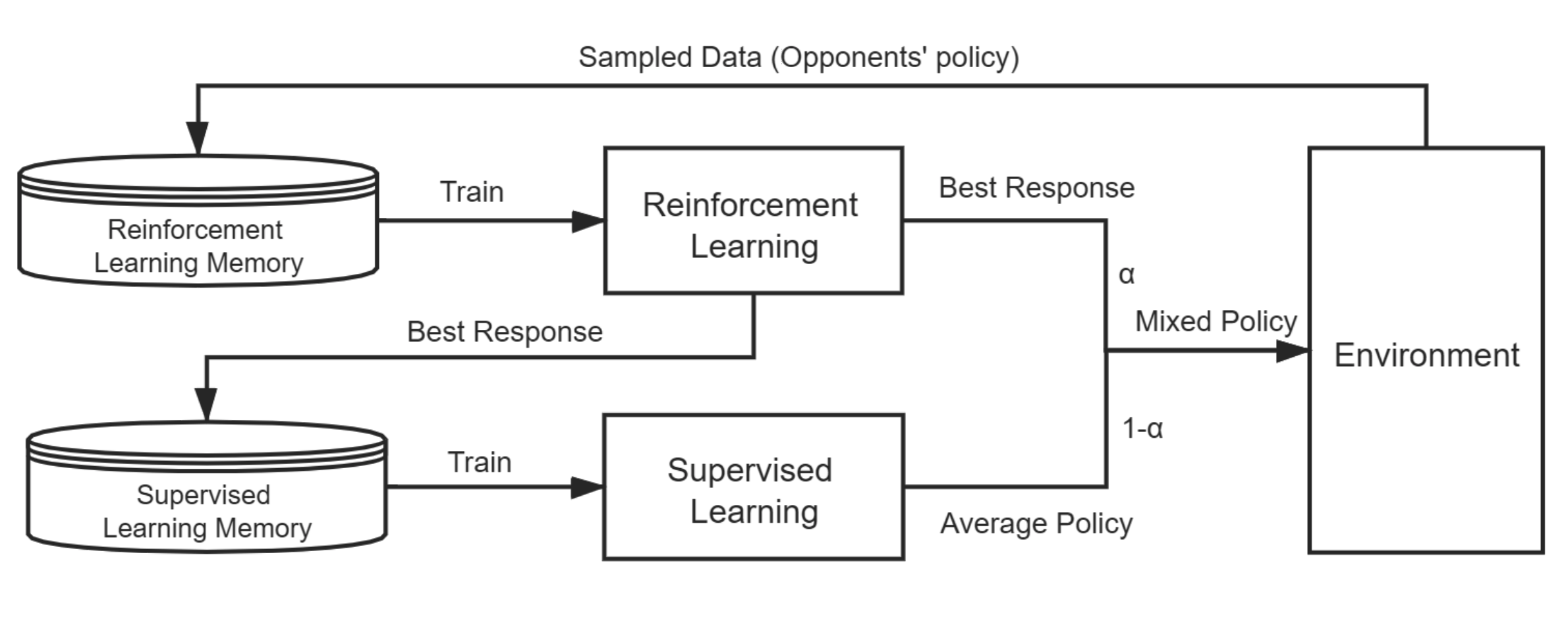 The overall structure of NFSP(one agent).
 In ReinforcementLearningZoo.jl, I implement the NFSPAgent which defines the NFSPAgent struct and designs its behaviors according to the NFSP algorithm, including collecting needed information and how to update the policy. And the NFSPAgentManager is a special multi-agent manager that all agents apply NFSP algorithm. Besides, in the abstract_nfsp, I customize the run function for NFSPAgentManager.
Since the core of the algorithm is to define the behavior of the NFSPAgent, I'll explain how it is done as the following:
mutable struct NFSPAgent <: AbstractPolicy
rl_agent::Agent
sl_agent::Agent
η
rng
update_freq::Int
update_step::Int
mode::Bool
end
Based on our discussion in section 2.1, the core of the NFSPAgent is to customize its behavior in different stages:
Here, the NFSPAgent should be set to the training mode based on the anticipatory dynamics. Besides, the terminated state and dummy action of the last episode must be removed at the beginning of each episode. (see the note)
function (π::NFSPAgent)(stage::PreEpisodeStage, env::AbstractEnv, ::Any)
update!(π.rl_agent.trajectory, π.rl_agent.policy, env, stage)
π.mode = rand(π.rng) < π.η
end
In this stage, the NFSPAgent should collect the personal information of state and action, and add them into the RL agent's trajectory. If it is set to the best response mode, we also need to update the SL agent's trajectory. Besides, if the condition of updating is satisfied, the inner agents also need to be updated. The code is just like the following:
function (π::NFSPAgent)(stage::PreActStage, env::AbstractEnv, action)
rl = π.rl_agent
sl = π.sl_agent
if π.mode
update!(sl.trajectory, sl.policy, env, stage, action)
rl(stage, env, action)
else
update!(rl.trajectory, rl.policy, env, stage, action)
end
π.update_step += 1
if π.update_step % π.update_freq == 0
if π.mode
update!(sl.policy, sl.trajectory)
else
rl_learn!(rl.policy, rl.trajectory)
update!(sl.policy, sl.trajectory)
end
end
end
After executing the action, the NFSPAgent needs to add the personal reward and the is_terminated results of the current state into the RL agent's trajectory.
function (π::NFSPAgent)(::PostActStage, env::AbstractEnv, player::Any)
    push!(π.rl_agent.trajectory[:reward], reward(env, player))
    push!(π.rl_agent.trajectory[:terminal], is_terminated(env))
end
When one episode is terminated, the agent should push the terminated state and a dummy action (see also the note) into the RL agent's trajectory. Also, the reward and is_terminated results need to be corrected to avoid getting the wrong samples when playing the games of SEQUENTIAL or TERMINAL_REWARD.
function (π::NFSPAgent)(::PostEpisodeStage, env::AbstractEnv, player::Any)
rl = π.rl_agent
sl = π.sl_agent
if !rl.trajectory[:terminal][end]
rl.trajectory[:reward][end] = reward(env, player)
rl.trajectory[:terminal][end] = is_terminated(env)
end
action = rand(action_space(env, player))
push!(rl.trajectory[:state], state(env, player))
push!(rl.trajectory[:action], action)
if haskey(rl.trajectory, :legal_actions_mask)
push!(rl.trajectory[:legal_actions_mask], legal_action_space_mask(env, player))
end
...
end
According to the paper, by default the RL agent is as QBasedPolicy with CircularArraySARTTrajectory. And the SL agent is default as BehaviorCloningPolicy with ReservoirTrajectory. So you can customize the agent under the restriction and test the algorithm on any interested multi-agent games. Note that if the game's states can't be used as the network's input, you need to add a state-related wrapper to the environment before applying the algorithm.
Here is one experiment JuliaRL_NFSP_KuhnPoker as one usage example, which tests the algorithm on the Kuhn Poker game. Since the type of states in the existing KuhnPokerEnv is the tuple of symbols, I simply encode the state just like the following:
env = KuhnPokerEnv()
wrapped_env = StateTransformedEnv(
    env;
    state_mapping = s -> [findfirst(==(s), state_space(env))],
    state_space_mapping = ss -> [[findfirst(==(s), state_space(env))] for s in state_space(env)]
    )
In this experiment, RL agent use DQNLearner to learn the best response:
rl_agent = Agent(
    policy = QBasedPolicy(
        learner = DQNLearner(
            approximator = NeuralNetworkApproximator(
                model = Chain(
                    Dense(ns, 64, relu; init = glorot_normal(rng)),
                    Dense(64, na; init = glorot_normal(rng))
                ) |> cpu,
                optimizer = Descent(0.01),
            ),
            target_approximator = NeuralNetworkApproximator(
                model = Chain(
                    Dense(ns, 64, relu; init = glorot_normal(rng)),
                    Dense(64, na; init = glorot_normal(rng))
                ) |> cpu,
            ),
            γ = 1.0f0,
            loss_func = huber_loss,
            batchsize = 128,
            update_freq = 128,
            min_replay_history = 1000,
            target_update_freq = 1000,
            rng = rng,
        ),
        explorer = EpsilonGreedyExplorer(
            kind = :linear,
            ϵ_init = 0.06,
            ϵ_stable = 0.001,
            decay_steps = 1_000_000,
            rng = rng,
        ),
    ),
    trajectory = CircularArraySARTTrajectory(
        capacity = 200_000,
        state = Vector{Int} => (ns, ),
    ),
)
And the SL agent is defined as the following:
sl_agent = Agent(
policy = BehaviorCloningPolicy(;
approximator = NeuralNetworkApproximator(
model = Chain(
Dense(ns, 64, relu; init = glorot_normal(rng)),
Dense(64, na; init = glorot_normal(rng))
) |> cpu,
optimizer = Descent(0.01),
),
explorer = WeightedSoftmaxExplorer(),
batchsize = 128,
min_reservoir_history = 1000,
rng = rng,
),
trajectory = ReservoirTrajectory(
2_000_000;
rng = rng,
:state => Vector{Int},
:action => Int,
),
)
Based on the defined inner agents, the NFSPAgentManager can be customized as the following:
nfsp = NFSPAgentManager(
Dict(
(player, NFSPAgent(
deepcopy(rl_agent),
deepcopy(sl_agent),
0.1f0,
rng,
128,
0,
true,
)) for player in players(wrapped_env) if player != chance_player(wrapped_env)
)
)
Based on the setting stop_condition and designed hook in the experiment, you can just run(nfsp, wrapped_env, stop_condition, hook) to perform the experiment. Use Plots.plot to get the following result:
 Play KuhnPoker with NFSP.
 Besides, you can also play games implemented in 3rd party OpenSpiel(see the doc) with NFSPAgentManager, such as "kuhn_poker" and "leduc_poker", just like the following:
env = OpenSpielEnv("kuhn_poker")
wrapped_env = ActionTransformedEnv(
env,
action_mapping = a -> RLBase.current_player(env) == chance_player(env) ? a : Int(a - 1),
action_space_mapping = as -> RLBase.current_player(env) == chance_player(env) ?
as : Base.OneTo(num_distinct_actions(env.game)),
)
wrapped_env = DefaultStateStyleEnv{InformationSet{Array}()}(wrapped_env)
Apart from the above environment wrapping, most details are the same with the experiment JuliaRL_NFSP_KuhnPoker. The result is shown below. For more details, you can refer to the experiment JuliaRL_NFSP_OpenSpiel(kuhn_poker).
.png) Play "kuhn_poker" in OpenSpiel with NFSP.
Play "kuhn_poker" in OpenSpiel with NFSP. The Multi-agent Deep Deterministic Policy Gradient(MADDPG) algorithm improves the Deep Deterministic Policy Gradient(DDPG), which also works well on multi-agent games. Based on the DDPG, the critic of each agent in MADDPG can get all agents' policies according to the paper's hypothesis, including their personal states and actions, which can help to get a more reasonable score of the actor's policy. The following figure(from the paper) illustrates the framework of MADDPG.
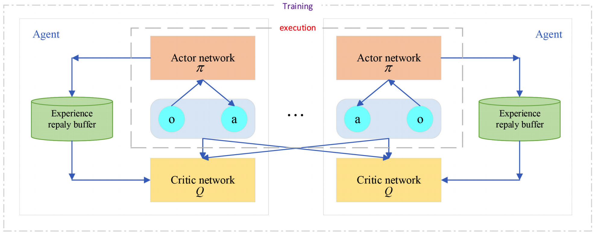 The framework of MADDPG.
 Given that the DDPGPolicy is already implemented in the ReinforcementLearningZoo.jl, I implement the MADDPGManager which is a special multi-agent manager that all agents apply DDPGPolicy with one improved critic. The structure of MADDPGManager is as the following:
mutable struct MADDPGManager <: AbstractPolicy
    agents::Dict{<:Any, <:Agent}
    traces
    batchsize::Int
    update_freq::Int
    update_step::Int
    rng::AbstractRNG
end
Each agent in the MADDPGManager uses DDPGPolicy with one trajectory, which collects their own information. Note that the policy of the Agent should be wrapped with NamedPolicy. NamedPolicy is a useful substruct of AbstractPolicy when meeting the multi-agent games, which combine the player's name and detailed policy. So that can use Agent 's default behaviors to collect the necessary information.
As for updating the policy, the process is mainly the same as the DDPGPolicy, apart from each agent's critic will assemble all agents' personal states and actions. For more details, you can refer to the code.
Note that when calculating the loss of actor's behavior network, we should add the reg term to improve the algorithm's performance, which differs from DDPG.
gs2 = gradient(Flux.params(A)) do
v = C(vcat(s, mu_actions)) |> vec
reg = mean(A(batches[player][:state]) .^ 2)
-mean(v) + reg * 1e-3
end
Here MADDPGManager is used for the environments of SIMULTANEOUS and continuous action space(see the blog Diagonal Gaussian Policies), or you can add an action-related wrapper to the environment to ensure it can work with the algorithm. There is one experiment JuliaRL_MADDPG_KuhnPoker as one usage example, which tests the algorithm on the Kuhn Poker game. Since the Kuhn Poker is one SEQUENTIAL game with discrete action space(see also the blog Diagonal Gaussian Policies), I wrap the environment just like the following:
wrapped_env = ActionTransformedEnv(
StateTransformedEnv(
env;
state_mapping = s -> [findfirst(==(s), state_space(env))],
state_space_mapping = ss -> [[findfirst(==(s), state_space(env))] for s in state_space(env)]
),
action_mapping = x -> length(x) == 1 ? x : Int(ceil(x[current_player(env)]) + 1),
)
And customize the following actor and critic's network:
rng = StableRNG(123)
ns, na = 1, 1
n_players = 2
create_actor() = Chain(
Dense(ns, 64, relu; init = glorot_uniform(rng)),
Dense(64, 64, relu; init = glorot_uniform(rng)),
Dense(64, na, tanh; init = glorot_uniform(rng)),
)
create_critic() = Chain(
Dense(n_players * ns + n_players * na, 64, relu; init = glorot_uniform(rng)),
Dense(64, 64, relu; init = glorot_uniform(rng)),
Dense(64, 1; init = glorot_uniform(rng)),
)
So that can design the inner DDPGPolicy and trajectory like the following:
policy = DDPGPolicy(
behavior_actor = NeuralNetworkApproximator(
model = create_actor(),
optimizer = Adam(),
),
behavior_critic = NeuralNetworkApproximator(
model = create_critic(),
optimizer = Adam(),
),
target_actor = NeuralNetworkApproximator(
model = create_actor(),
optimizer = Adam(),
),
target_critic = NeuralNetworkApproximator(
model = create_critic(),
optimizer = Adam(),
),
γ = 0.95f0,
ρ = 0.99f0,
na = na,
start_steps = 1000,
start_policy = RandomPolicy(-0.99..0.99; rng = rng),
update_after = 1000,
act_limit = 0.99,
act_noise = 0.,
rng = rng,
)
trajectory = CircularArraySARTTrajectory(
capacity = 100_000,
state = Vector{Int} => (ns, ),
action = Float32 => (na, ),
)
Based on the above policy and trajectory, the MADDPGManager can be defined as the following:
agents = MADDPGManager(
Dict((player, Agent(
policy = NamedPolicy(player, deepcopy(policy)),
trajectory = deepcopy(trajectory),
)) for player in players(env) if player != chance_player(env)),
SARTS,
512,
100,
0,
rng
)
Plus on the stop_condition and hook in the experiment, you can also run(agents, wrapped_env, stop_condition, hook) to perform the experiment. Use Plots.scatter to get the following result:
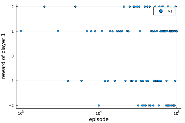 Play KuhnPoker with MADDPG.
 However, KuhnPoker is not a good choice to show the performance of MADDPG. For testing the algorithm, I add SpeakerListenerEnv into ReinforcementLearningEnvironments.jl, which is a simple cooperative multi-agent game.
Since two players have different dimensions of state and action in the SpeakerListenerEnv, the policy and the trajectory are customized as below:
env = SpeakerListenerEnv(max_steps = 25)
init = glorot_uniform(rng)
critic_dim = sum(length(state(env, p)) + length(action_space(env, p)) for p in (:Speaker, :Listener))
create_actor(player) = Chain(
Dense(length(state(env, player)), 64, relu; init = init),
Dense(64, 64, relu; init = init),
Dense(64, length(action_space(env, player)); init = init)
)
create_critic(critic_dim) = Chain(
Dense(critic_dim, 64, relu; init = init),
Dense(64, 64, relu; init = init),
Dense(64, 1; init = init),
)
create_policy(player) = DDPGPolicy(
behavior_actor = NeuralNetworkApproximator(
model = create_actor(player),
optimizer = OptimiserChain(ClipNorm(0.5), Adam(1e-2)),
),
behavior_critic = NeuralNetworkApproximator(
model = create_critic(critic_dim),
optimizer = OptimiserChain(ClipNorm(0.5), Adam(1e-2)),
),
target_actor = NeuralNetworkApproximator(
model = create_actor(player),
),
target_critic = NeuralNetworkApproximator(
model = create_critic(critic_dim),
),
γ = 0.95f0,
ρ = 0.99f0,
na = length(action_space(env, player)),
start_steps = 0,
start_policy = nothing,
update_after = 512 * env.max_steps,
act_limit = 1.0,
act_noise = 0.,
)
create_trajectory(player) = CircularArraySARTTrajectory(
capacity = 1_000_000,
state = Vector{Float64} => (length(state(env, player)), ),
action = Vector{Float64} => (length(action_space(env, player)), ),
)
Based on the above policy and trajectory, we can design the corresponding MADDPGManager:
agents = MADDPGManager(
Dict(
player => Agent(
policy = NamedPolicy(player, create_policy(player)),
trajectory = create_trajectory(player),
) for player in (:Speaker, :Listener)
),
SARTS,
512,
100,
0,
rng
)
Add the stop_condition and designed hook, we can simply run(agents, env, stop_condition, hook) to run the experiment and use Plots.plot to get the following result.
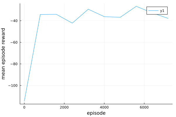 Play SpeakerListenerEnv with MADDPG.
 Exploitability Descent(ED) is the algorithm to compute approximate equilibria in two-player zero-sum extensive-form games with imperfect information. The ED algorithm directly optimizes the player's policy against the worst case oppoent. The exploitability of each player applying ED's policy converges asymptotically to zero. Hence in self-play, the joint policy π converges to an approximate Nash Equilibrium.
Unlike the above two algorithms, the ED algorithm does not need to collect the information in each stage. Instead, on each iteration, there are the following two steps that occur for each player employing the ED algorithm:
Compute the best response policy to each player's policy;
Perform the gradient ascent on the policy to increase each player's utility against the respective best responder(i.e. the opponent), which aims to decrease each player's exploitability.
In ReinforcementLearingZoo.jl, I implement EDPolicy which defines the EDPolicy struct and customize the interactions with the environments:
mutable struct EDPolicy{P<:NeuralNetworkApproximator, E<:AbstractExplorer}
opponent::Any
learner::P
explorer::E
end
function (π::EDPolicy)(env::AbstractEnv)
s = state(env)
s = send_to_device(device(π.learner), Flux.unsqueeze(s, ndims(s) + 1))
logits = π.learner(s) |> vec |> send_to_host
ActionStyle(env) isa MinimalActionSet ? π.explorer(logits) :
π.explorer(logits, legal_action_space_mask(env))
end
_device(π::EDPolicy, x) = send_to_device(device(π.learner), x)
function RLBase.prob(π::EDPolicy, env::AbstractEnv; to_host::Bool = true)
s = @ignore state(env) |> x -> Flux.unsqueeze(x, ndims(x) + 1) |> x -> _device(π, x)
logits = π.learner(s) |> vec
mask = @ignore legal_action_space_mask(env) |> x -> _device(π, x)
p = ActionStyle(env) isa MinimalActionSet ? prob(π.explorer, logits) : prob(π.explorer, logits, mask)
to_host ? p |> send_to_host : p
end
function RLBase.prob(π::EDPolicy, env::AbstractEnv, action)
A = action_space(env)
P = prob(π, env)
@assert length(A) == length(P)
if A isa Base.OneTo
P[action]
else
for (a, p) in zip(A, P)
if a == action
return p
end
end
@error "action[$action] is not found in action space[$(action_space(env))]"
end
end
Here I use many macro operators @ignore for being able to compute the gradient of the parameters. Also, I design the update! function for EDPolicy when getting the opponent's best response policy:
function RLBase.update!(
π::EDPolicy,
Opponent_BR::BestResponsePolicy,
env::AbstractEnv,
player::Any,
)
reset!(env)
policy_vs_br = PolicyVsBestReponse(
MultiAgentManager(
NamedPolicy(player, π),
NamedPolicy(π.opponent, Opponent_BR),
),
env,
player,
)
info_states = collect(keys(policy_vs_br.info_reach_prob))
cfr_reach_prob = collect(values(policy_vs_br.info_reach_prob)) |> x -> _device(π, x)
gs = gradient(Flux.params(π.learner)) do
baseline = @ignore stack(([values_vs_br(policy_vs_br, e)] for e in info_states); dims=1) |> x -> _device(π, x)
q_values = stack((q_value(π, policy_vs_br, e) for e in info_states); dims=1)
advantage = q_values .- baseline
policy_values = stack((prob(π, e, to_host = false) for e in info_states); dims=1)
loss_per_state = - sum(policy_values .* advantage, dims = 2)
sum(loss_per_state .* cfr_reach_prob)
end
update!(π.learner, gs)
end
Here I implement one PolicyVsBestResponse struct for computing related values, such as the probabilities of opponent's reaching one particular environment in playing, and the expected reward from the start of a specific environment when against the opponent's best response.
Besides, I implement the EDManager, which is a special multi-agent manager that all agents utilize the ED algorithm, and set the particular run function for running the experiment:
function Base.run(
π::EDManager,
env::AbstractEnv,
stop_condition = StopAfterNEpisodes(1),
hook::AbstractHook = EmptyHook(),
)
@assert NumAgentStyle(env) == MultiAgent(2) "ED algorithm only support 2-players games."
@assert UtilityStyle(env) isa ZeroSum "ED algorithm only support zero-sum games."
is_stop = false
while !is_stop
RLBase.reset!(env)
hook(PRE_EPISODE_STAGE, π, env)
for (player, policy) in π.agents
oppo_best_response = BestResponsePolicy(π, env, policy.opponent)
update!(policy, oppo_best_response, env, player)
end
RLBase.reset!(env)
while !is_terminated(env)
π(env) |> env
end
if stop_condition(π, env)
is_stop = true
break
end
hook(POST_EPISODE_STAGE, π, env)
end
hook(POST_EXPERIMENT_STAGE, π, env)
hook
end
According to the paper, EDmanager only supports for the two-player zero-sum games. There is one experiment JuliaRL_ED_OpenSpiel as one usage example, which tests the algorithm on the Kuhn Poker game in 3rd-party OpenSpiel. Here I also customized the hook and stop_condition for testing the implemented ED algorithm.
New hook is designed as the following:
mutable struct KuhnOpenNewEDHook <: AbstractHook
episode::Int
eval_freq::Int
episodes::Vector{Int}
results::Vector{Float64}
end
function (hook::KuhnOpenNewEDHook)(::PreEpisodeStage, policy, env)
hook.episode += 1
if hook.episode % hook.eval_freq == 1
push!(hook.episodes, hook.episode)
push!(hook.results, RLZoo.nash_conv(policy, env))
end
for (_, agent) in policy.agents
agent.learner.optimizer[2].eta = 1.0 / sqrt(hook.episode)
end
end
Next, wrap the environment and initialize the EDmanager, hook and stop_condition:
rng = StableRNG(123)
env = OpenSpielEnv(game)
wrapped_env = ActionTransformedEnv(
env,
action_mapping = a -> RLBase.current_player(env) == chance_player(env) ? a : Int(a - 1),
action_space_mapping = as -> RLBase.current_player(env) == chance_player(env) ?
as : Base.OneTo(num_distinct_actions(env.game)),
)
wrapped_env = DefaultStateStyleEnv{InformationSet{Array}()}(wrapped_env)
player = 0
ns, na = length(state(wrapped_env, player)), length(action_space(wrapped_env, player))
create_network() = Chain(
Dense(ns, 64, relu;init = glorot_uniform(rng)),
Dense(64, na;init = glorot_uniform(rng))
)
create_learner() = NeuralNetworkApproximator(
model = create_network(),
optimizer = Flux.Optimise.Optimiser(WeightDecay(0.001), Descent())
)
EDmanager = EDManager(
Dict(
player => EDPolicy(
1 - player,
create_learner(),
WeightedSoftmaxExplorer(),
) for player in players(env) if player != chance_player(env)
)
)
stop_condition = StopAfterNEpisodes(100_000, is_show_progress=!haskey(ENV, "CI"))
hook = KuhnOpenNewEDHook(0, 100, [], [])
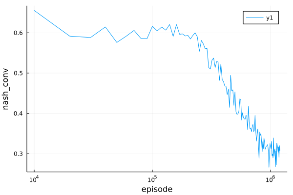
Based on the above setting, you can perform the experiment by run(EDmanager, wrapped_env, stop_condition, hook). Use the following Plots.plot to get the experiment's result:
plot(hook.episodes, hook.results, scale=:log10, xlabel="episode", ylabel="nash_conv")
.png) Play "kuhn_poker" in OpenSpiel with ED.
Play "kuhn_poker" in OpenSpiel with ED.