The goal of ReinforcementLearning.jl is to provide a collection of tools for learning and implementing reinforcement learning algorithms. This means that, unlike many other existing packages focusing on deep reinforcement learning only, we aim to build a rich ecosystem to solve different kinds of tasks in reinforcement learning, including but not limited to the following fields:
Tabular reinforcement learning
Deep reinforcement learning
Offline reinforcement learning
Multi-agent reinforcement learning
Model-based reinforcement learning
Although most existing reinforcement learning related packages are written in Python with PyTorch or Tensorflow as the backend, we choose Julia because of the following advantages:
Multiple dispatch in Julia makes the code very easy to read, understand and extend. Without this feature, it's hard to imagine how to organize such a package targeting so many different tasks in an elegant way.
Composable Multi-threading boost the speed of interactions between agents and environments.
Julia is fast and easy to interact with other programming languages like Python, C, C++, fortran so that we can easily leverage many existing packages.
Many existing packages inspired the development of ReinforcementLearning.jl a lot. Following are some important ones.
Dopamine provides a clear implementation of the Rainbow algorithm. The gin config file template and the concise workflow is the origin of the Experiment in ReinforcementLearning.jl.
OpenSpiel provides a lot of useful functions to describe many different kinds of games. They are turned into traits in our package.
Ray/rllib has many nice abstraction layers in the policy part. We also borrowed the definition of environments here. This is explained with details in section 2.
rlpyt has a nice code structure and we borrowed some implementations of policy gradient algorithms from it.
Acme offers a framework for distributed reinforcement learning.
The standard setting for reinforcement learning contains two parts: Agent and Environment. To make things general enough, we defined two abstract types: AbstractPolicy and AbstractEnv correspondingly.
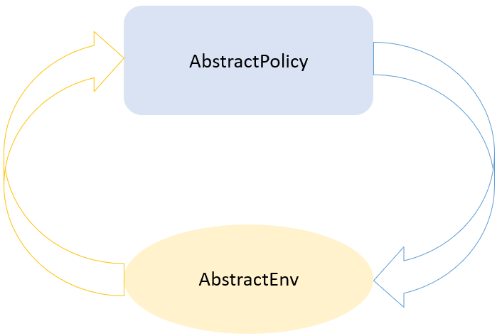 A general workflow between policy and environment.
 Figure 1: The general flow between a policy and an environment.
A policy simply takes a look at the environment and yields an action. And an environment will modify its internal state once received an action. So for continuing tasks, we can describe the workflow with the following code:
function Base.run(policy, env)
    while true
        env |> policy |> env
    end
end
For episodic tasks, two extra methods must be implemented for the env:
Then we have the following code:
function Base.run(policy, env)
    while true
        reset!(env)
        while !is_terminated(env)
            env |> policy |> env
        end
    end
end
In real world tasks, we never expect the workflow to run infinitely. Usually we will stop early after a number of steps/episodes or when the policy or environment meet some specific condition. Now let's introduce a stop_condition which examines policy and env after each step to control the workflow.
function Base.run(policy, env, stop_condition)
    while true
        reset!(env)
        while !is_terminated(env)
            env |> policy |> env
            stop_condition(policy, env) && return
        end
    end
end
Until now, a policy is still very general. We don't know it's actually updating or exploiting. However, in most cases, if a policy needs to be updated during interactions with the environment, it needs a buffer to collect some necessary information and then use it to update its strategy at some time. So a special policy named Agent is provided in our package to help update a policy.
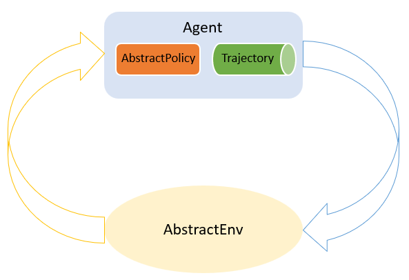 An illustration of Agent.
 An agent is simply a combination of any policy to be updated and a corresponding experience replay buffer (we call it AbstractTrajectory ). And we split the above workflow into the following stages to allow injecting different updating logics:
PreExperimentStage
PreEpisodeStage
PreActStage
PostActStage
PostEpisodeStage
PostExperimentStage
function Base.run(policy, env, stop_condition)
    while true
        reset!(env)
        policy(PRE_EPISODE_STAGE, env)
        while !is_terminated(env)
            action = policy(env)
            policy(PRE_ACT_STAGE, env, action)
            env(action)
            policy(POST_ACT_STAGE, env)
            stop_condition(policy, env) && return
        end
        policy(POST_EPISODE_STAGE, env)
    end
end
Note that by default, update!(policy::AbstractPolicy, ::AbstractStage, env) will do nothing and the workflow is simplified to the earlier version. For the specific policy Agent, it will update its internal policy and trajectory at each stage:
update!(policy, trajectory, env, stage) (Read as update! the inner policy given a trajectory, env and the current stage)
update!(trajectory, policy, env, stage) (Read as update! the inner trajectory given a policy, env and the current stage)
update!(trajectory, policy, env, ::PreActStage, action) (The action here is the one selected by the policy to be executed on the env)
By default, update!(policy, trajectory, env, stage) will do nothing. The default implementation of update!(trajectory, policy, env, stage) is explained in the 2.2 Trajectory section. But developers can customize these behaviors easily thanks to multiple dispatch.
Now the policy can play happily with the environment. We would also want to inject some meaningful actions in the meantime. For example, collecting the total reward of each episode, logging the loss of each updating, saving the policy periodically, modifying some hyperparameters on the fly and so on. So a general callback is introduced.
function Base.run(policy, env, stop_condition, hook)
    hook(PRE_EXPERIMENT_STAGE, env)
    while true
        reset!(env)
        policy(PRE_EPISODE_STAGE, env)
        hook(PRE_EPISODE_STAGE, env)
        while !is_terminated(env)
            action = policy(env)
            policy(PRE_ACT_STAGE, env, action)
            hook(PRE_ACT_STAGE, env, action)
            env(action)
            policy(POST_ACT_STAGE, env)
            hook(POST_ACT_STAGE, env)
            stop_condition(policy, env) && return
        end
        policy(POST_EPISODE_STAGE, env)
        hook(POST_EPISODE_STAGE, env)
    end
end
Except for some corner cases, the code above is very close to our implementation.
We use the AbstractTrajectory to describe the container used to collect intermediate data during the interactions between policy and environment. Among all the different implementations, the simplest one is Trajectory. Essentially, it's just a wrapper of a NamedTuple with some customized behaviors to avoid type piracy.
 The default implementation of
 VectorSARTTrajectory. The above figure illustrates the simplest trajectory: VectorSARTTrajectory. It contains four traces: state, action, reward and terminal. Each trace simply use a Vector as the container. By default, the trajectory is assumed to be of the SARTSA format (State, Action, Reward, Termination, next-State, next-Action). For different policies, developers may replace the inner container, add/remove traces or customize the inserting/removing/sampling strategy. All the available built-in trajectories can be found here.
For environments with a small state space, we can use a table to record the state value, state-action value (or any other values we are interested in). While in environments with a large state space, we often use a neural network to estimate the values nowadays. To generalize these two cases, an AbstractApproximator is introduced. Basically it's just parameters (either tabular or neural network based) plus an optimizer. Another benefit of introducing such a layer is to hide the underlying DNN framework from developers so that we can easily switch from Flux.jl to Knet.jl or something else.
In this section, we'll give a brief introduction to different types of reinforcement learning algorithms implemented in our package. After that we'll relate these algorithms with the underlying components provided in our package. Developers should feel confident to implement new algorithms after reading this section. Note that all the code snippets here are for illustration only, they may differ from the one provided in the package.
Following the standard textbook definitions, the interactions between an agent and environment can be formalized as a fully-observable or partially-observable Markov decision process ((PO)MDP). Here we focus on the fully-observable MDP. The MDP is defined as a tuple M=(S,A,T,d0,r,γ) where
S is a set of states s∈S
A is a set of actions
T is a conditional probability distribution T(st+1∣st,at)
d0 is the initial state distribution of s0
r is a reward function: S×A→R
γ∈(0,1] is a scalar discount factor
At each time t, the policy π takes a look at the current state of the environment st and produces an action at=π(st). After taking this action, we can fetch reward rt=r(st,at), next state st+1 and the episode termination signal et from the environment. The basic transition in each step is τ=(st,at,rt,e0,st+1,at+1), which forms the trajectory T=(st,at,rt,e0,...,sH,aH) of VectorSARTTrajectory we mentioned above. The trajectory distribution pπ for a given MDP M and policy π is given by
pπ(T)=d0(s0)t=0∏Hπ(at∣st)T(st+1∣st,at) The only goal in reinforcement learning is to maximize some form of the expected return. And we focus on the discounted rewards below
Rt=i≥0∑γirt=rt+γRt+1 Note that if we can estimate the state value or state-action value accurately, it will be easy to get a near-optimal policy. The state value function Vπ(st) estimates the return Rt by following the policy π starting from state st:
Vπ(st)=ET∼pπ(T∣st)Rt Similarly, for state action value function Qπ(st,at), it estimates Rt by following the policy π starting from a state-action pair (st,at):
Qπ(st,at)=ET∼pπ(T∣st,at)Rt We can derive the recursive definitions of these two functions:
Vπ(st)=Eat∼π(at∣st)[Qπ(st,at)] Qπ(st,at)=r(st,at)+γEst+1∼T(st+1∣st,at)[Vπ(st+1)] And combining the above two equations, we can describe Qπ(st,at) in terms of Qπ(st+1,at+1):
Qπ(st,at)=r(st,at)+γEst+1∼T(st+1∣st,at),at+1∼π(at+1∣st+1)[Qπ(st+1,at+1)] With the policy of Q-function, π(at∣st)=atargmax Q(st,at), we have the following condition on the optimal Q-function:
Q⋆(st,at)=r(st,at)+γEst+1∼T(st+1∣st,at)[at+1max Q⋆(st+1,at+1)] To estimate the state value of some specific policy Vπ, a VBasedPolicy is provided in our package:
struct VBasedPolicy{L,M} <: AbstractPolicy
    learner::L
    mapper::M
end

RLBase.plan!(p::VBasedPolicy, env::AbstractEnv) = p.mapper(env, p.learner)
Basically it contains two parts, a value learner V and a mapper policy π. And all the updating to this policy will be forwarded to the inner learner.
Monte Carlo Prediction for Estimating Vπ
Now let's start from a very basic value learner, the Monte Carlo based value learner. The idea is to apply the VBasedPolicy until the end of an episode. And update the value estimation of each state with the accumulated averaging R(s). There're two steps involved in implementing such a learner:
Updating the trajectory
Updating the learner
By default, the VectorSARTTrajectory we've seen above will add all the transitions into it. But this is not what we want in the Monte Carlo based value learner here. We only need one episode actually. So we can empty the trajectory at the beginning of each episode by implementing:
RLBase.update!(
    t::AbstractTrajectory,
    ::VBasedPolicy{MCLearner},
    ::AbstractEnv,
    ::PreEpisodeStage
)
    empty!(t)
end
Next, we update the learner only at the end of an episode. So we have the following method implemented:
RLBase.update!(
::MCLearner,
::AbstractTrajectory,
::AbstractEnv,
::PostEpisodeStage
)
end
Tabular TD(0) for estimating Vπ
Another approach to estimate the value function is to use the zero step temporal-difference learning. The main difference compared to the MC method above is that, now we update the learner and trajectory at the PostActStage and PostEpisodeStage.
In our package, the QBasedPolicy is provided for all the general Q function based policies. It consists of a Q value learner and an explorer to select action based on the estimated Q value.
struct QBasedPolicy{L, E} <: AbstractPolicy
    learner::L
    explorer::E
end

RLBase.plan!((p::QBasedPolicy, env::AbstractEnv) = env |> p.learner |> p.explorer
Similar to the VBasedPolicy, when wrapped in an Agent, all updating to QBasedPolicy will be forwarded to the inner value learner.
TabularQLearning
For tabular Q-learning, we use a TabularQApproximator to estimate the Q(st,at). At each PostActStage, we calculate the TD error:
δ=rt+γat+1∼π(at+1∣st+1)maxQ(st+1,at+1)−Q(st,at) And use it to update the inner TabularApproximator. From the API implementation level, if the QBasedPolicy{<:TabularQLearner} is used together with a VectorSARTTrajectory like we mentioned above, then we should remember to empty the trajectory at the end of each episode.
BasicDQN
To tackle problems with a large state space, a neural network Qϕ is used to estimate the Qπ where ϕ is the parameters. To optimize the parameters, we can optimize the loss function of Li(ϕi) at each PreActStage i:
Li(ϕi)=Es,a∼T[(yi(s,a)−Qϕi(s,a))2] where yi is a bootstrap target:
yi(s,a)=Es′∼T(s,a)[r+γa′∼π(s′)maxQϕi−1(s′,a′)] Compared to TabularQLearning, we need the following modifications:
A CircularArraySARTTrajectory is used instead of VectorSARTTrajectory
The TabularApproximator is replaced with NeuralNetworkApproximator
Since DQN and its variants usually need to sample minibatches from a trajectory, inspired by adders and inserters in Acme, we also exported some AbstractSampler . Users may refer the source code for some extra enhancements like double-dqn and n-step dqn.
Prioritized DQN
The biggest challenge to implement Prioritized DQN is to create a new Trajectory. Fortunately, adding a new trace is pretty simple given that a Trajectory is merely a wrapper of a NamedTuple. To make sure each transition is inserted correctly, developers should carefully examine all the default implementations of update!(trajectory, policy, env, stage) and write your more specific ones when needed. For Prioritized DQN, we need to insert a default priority at the PostActStage. When updating the inner learner, we also need to update the priority trace.
IQN
For distributional reinforcement learning algorithms like C51 and IQN, the estimation is not the Q-values directly. But we can still fit them into the QBasedPolicy. The main change is to override the default implementation of RLBase.plan!((p::QBasedPolicy, env::AbstractEnv) to use the Q value distribution.
This article already gives a detailed explanation to a lot of policy gradient algorithms. Here we only describe some notable points to implement them. Some of the implemented policies (for example PPO) are very interesting and worth explaining them in detail in another blog later.
MultiThreadEnv
Except for some Monte Carlo based policy gradient algorithms (like Vanilla Policy Gradient), we usually roll out several simulations simultaneously and collect the transitions every n steps to train the policies. So this special environment wrapper is introduced to run several copies of environments by leveraging multi-threading. This environment breaks the workflow we defined before because is_terminated(::MultiThreadEnv) doesn't return a bool value any more. Also, the PreEpisodeStage and PostEpisodeStage are not valid. So a more specific implementation is defined.
function RLCore._run(
    policy::AbstractPolicy,
    env::MultiThreadEnv,
    stop_condition,
    hook::AbstractHook,
)

    while true
        action = policy(env)
        policy(PRE_ACT_STAGE, env, action)
        hook(PRE_ACT_STAGE, policy, env, action)

        env(action)

        policy(POST_ACT_STAGE, env)
        hook(POST_ACT_STAGE, policy, env)

        if stop_condition(policy, env)
            break
        end
    end
end
And the corresponding updating to the trajectory is also provided by default.
In offline reinforcement learning, we often assume the experience is prepared ahead. To adapt some of the above algorithms in the offline setting, we need to provide a more specific implementation of update!(policy, batch) and reuse it in update!(policy, trajectory, env stage) . For new offline algorithms, we only need to implement the following two methods:
RLBase.plan!((p::YourOfflinePolicy, env::AbstreactEnv)
update!(p::YourOfflinePolicy, batch)
In our initial workflow, there's only one agent interacting with the environment. To expand it to the multi-agent setting, a policy wrapper of MultiAgentPolicy and MultiAgentHook is added. At each stage, it fetches necessary information and forward the env to its children. Then based on the current player of the env, it selects the right child and generate an action properly.
There are two MultiAgent cases, Sequential and Simultaneous. For Sequential environments, RLBase.next_player! and current_player must be implemented so that the Base.run loop knows the order of play. For Simultaneous, the working assumption is that all players provided in MultiAgentPolicy play every turn. Two basic examples are provided, TicTacToeEnv and RockPaperScissorsEnv.
For each policy in our package, we provide at least an Experiment to make sure it works in some basic experiments or reproduces the results in the original paper. A thorough report will be provided soon after Julia@v1.6 is released.
It's hard to imagine that it's been years since we created this package. The following tips are what we learned during this period:
Keep interfaces simple and minimal
Adding new APIs is very cheap, but soon you will be the only one who knows how to use them. Keeping APIs simple and minimal will force you rethink your existing design and come up with a more natural one. Actually, the multi-dispatch in Julia encourages you to generalize the interfaces as much as possible.
Design early and refactor frequently
Once started coding, things will evolve very quickly. Focusing on new features only will introduce a lot of ad-hoc workarounds on the old design. To keep the system flexible, always remember to reserve some time for refactoring.
”Premature optimization is the root of all evil!“
In most cases, the overall simplicity is more important than speed. With multiple dispatch, it's always relatively easy to come up with a more efficient implementation without loss of generality.
Maintain a set of reproducible experiments
For experiments that can be finished in minutes, we should add them into tests and make sure they produce the same result after each PR. For large experiments, it's a good practice to run them after each patch release.
We've witnessed the fast development of the reinforcement learning field in the last several years. A lot of interesting algorithms are not included yet so contributions are always welcomed.